Conditional Formulas

Formulas that return field values based on specific conditions, for example, returning “Yes” when the condition is met or summing the values of fields that match the criteria.

List of Formulas

Below is the list of the supported formulas. Please note that the following formulas are case-sensitive.

Formula	Description
IF(value==condition,value_if_true,value_if_false)	Returns one value if the condition evaluates to TRUE, or another value if the condition evaluates to FALSE. For details, click here.
IFS(value=condition1,value_if_true1,value=condition2,value_if_true2,...,true,default value)	Check whether one or more conditions are met and return a value that corresponds to the first TRUE condition. For details, click here.
LOOKUP(value,lookup_list,[result_list])	Searches for the value in a one-column or one-row range (lookup_list), and returns the corresponding value from another one-column or one-row range (result_list). For details, click here.
AND(logical1, [logical2], ...)	Returns TRUE if all its conditions evaluate to TRUE; returns FALSE if one or more conditions evaluate to FALSE. For details, click here.
OR(logical1, [logical2], ...)	Returns TRUE if any condition is TRUE; returns FALSE if all conditions are FALSE. For details, click here.
NOT(logical)	Returns TRUE if the test condition is FALSE, and FALSE if the condition is TRUE. For details, click here.
UPDATEIF(condition,value_if_true)	Modifies a field value when at least one condition is met. For details, click here
COUNTIF(criteria_range,criteria)	Returns the number of values in a range within a Subtable field that meet a single specified criterion. For details, click here.
COUNTIFS(criteria_range1,criteria1,[criteria_range2,criteria2]...)	Applies criteria to Subtable fields across multiple ranges and counts the number of times all criteria are met. For details, click here.
SUMIF(range,criteria,[sum_range])	Returns the sum of values in a Subtable that meet a specified criterion. For details, click here.
SUMIFS(sum_range,criteria_range1,criteria1,[criteria_range2, criteria2],...)	Returns the sum of values in a Subtable where each row meets multiple criteria. For details, click here.
MAXIFS(max_range, criteria_range1, criteria1, [criteria_range2, criteria2], ...)	Returns the maximum value in a Subtable among cells that meet the specified conditions or criteria. For details, click here.
MINIFS(min_range, criteria_range1, criteria1, [criteria_range2, criteria2], ...)	Returns the minimum value in a Subtable among cells that meet the specified conditions or criteria. For details, click here.

Formula Usage Guide

Ragic supports the use of conditional formulas. Please be reminded that changing the Field Type may affect the calculation results in some situations.

Note: These are the two circumstances in which you'll need to add ".RAW" to the referenced field upon assigning the conditional formulas:

1. When using the operator "=" to reference two fields that equal the condition of the formula. However, when referring to only one field that equals a fixed value, ".RAW" is not needed.

2. When assigning the formula to a Numeric field using the operator "=" to reference a string field(text, selection, date, etc.) that equals a fixed string value (which will return a numeric value as a result). If you are referencing one Numeric field that equals a value with operator "=", ".RAW" is not needed.

For more details about ".RAW" please refer to this section.

Date fields are calculated as days.

Conditional formulas can also be nested.

IF Function Details and Applications

IF Function: Conditional Evaluation

The IF function returns one value if a specified condition evaluates to TRUE, and another value if it evaluates to FALSE.

Formula	Syntax
IF	IF(value==condition,value_if_true,value_if_false)

Examples:

Basic example: IF(A2==10,10,0)

If the value in the reference field A2 is equal to 10, the value in this field would be 10. For any other value of A2, the value of this field will be 0.

Having a string value as a result: IF(A1==1,'True','False')

If the value in the reference field A1 is equal to 1, the value in this field would be "True". For any other value of A1, the value of this field will be "False".

Practical usage: IF(A2>=60,'Yes','No')

If the age field is greater than or equal to 60, the value in this field "Qualifies for senior discount?" would be "Yes"; otherwise, the value would be "No".

Note:

Usage of the older syntax of the IF function in Ragic is still supported.

Value=='condition'?'value_if_true':'value_if_false'

Basic Example: A1=='open'?'O':'C'

If A1 is open, give O. If not, give C.

When to add .RAW?

1. Referencing two fields that are equal with the IF function

If you would like to reference two fields that are equal to each other with the operator "=" as the condition in conditional formulas, please add .RAW after the referenced fields.

Syntax
IF(field1.RAW=field2.RAW,value_if_true,value_if_false)

Examples:

Basic Example 1: IF(A1.RAW=A2.RAW,1,0)

If the value in the referenced field A1 equals the value in field A2, return 1, otherwise return 0.

Basic Example 2: IF(A1.RAW=A2.RAW,'Open','Closed')

If the value in the referenced field A1 equals the value in field A2, return "Open", otherwise return "Closed".

2. Referencing a string field that equals a fixed string value as the condition with the IF function

Syntax
IF(string_field1.RAW="string",numeric_value_if_true,numeric_value_if_false)

Example: IF(A1.RAW="Yes",1,0)

If the value in the referenced string field A1 equals "Yes", return 1, otherwise return 0.

If you are referencing one Numeric field that equals a value with operator "=", ".RAW" is not needed.

Example:IF(A1=1,'YES','NO')

If the value in the referenced field A1 equals 1, return "YES", otherwise return "NO".

3. Determining Whether a Field is Empty or Not

If you would like to use a formula to check whether a field is empty or not, your formula must add .RAW after the referenced field.

For example, the formula IF(A8.RAW='',"TRUE","FALSE") is used to check if the field on cell A8 is empty, and that field's value may be 0. Therefore, .RAW should be added.

Note: Without adding .RAW to your referenced field on your formula, the numerical value "0" will also be considered as an empty value.

4. Referencing the numeric value of a free text field and returning it as a text string

For example, if the field on A1 is a free text field with the numeric value "10001", and the field on A2 is a linked field with a conditional formula set to reference and return A1's value "10001", the formula would need to be set as the following: IF(A1!='', A1.RAW)

IF Function: Retrieving Text

If you would like to retrieve text from referenced fields by using the functions LEFT(), RIGHT(), and MID(), please add +"" after the field you're referencing.

Example:

IF(A1="Yes",A5,LEFT(A5+"",2))

If the value in the referenced field A1 is equal to "Yes", the value in this field would be the field value of A5. For any other value of A1, the value of this field will be the first 2 digits of A5.

IF Function: Referencing TODAY() or NOW()

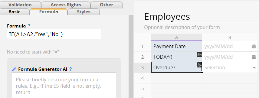
Since the system does not support referencing the value of TODAY() or NOW() within an IF() formula directly, you'll need to create another field that references a field containing the value of TODAY() or NOW().

Example:

If you want to compare the value of the date field A1 to TODAY(), you can create field A2 and configure it with TODAY(). Then, apply the formula: IF(A1>A2,"Valid","Expired")

If the value in the reference field A1 is larger than TODAY(), the value in this field would be "Valid". For a value that is smaller than TODAY(), the value of this field will be "Expired".

On the other hand, if you want to use the TODAY() formula or the field assigned the TODAY() formula as the referenced conditional field for calculations in IF() formulas, you can create field A2 for whole calculations as follows: A1-TODAY(). Then, apply the formula: IF(A2>0,"Valid","Expired")

Note: The value of TODAY() or NOW() will not be auto-recalculated once the entries are saved. If it's necessary to recalculate the TODAY() or NOW() value, you'll need to Apply a Daily Workflow.

IF Function: Referencing a Date Field

1. Apply on the non-Date field to compare the values of Date fields

For example, A1 and A2 are date fields, applying TODAY() to A2. In A4, enter the formula: IF(A1>A2,"Yes","No")

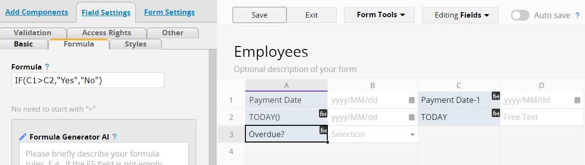
2. Apply on Numeric fields to execute addition or subtraction operations for Date fields

For example, it's not supported to enter the formula IF(A1-1>A2,"Yes","No") in A4. You will need to create the other two numeric fields C1 and C2. In C1, enter the formual: A1-1. In C2, enter A2. In A4, change the formula to IF(C1>C2,"Yes","No").

Subtable Conditional Formulas

COUNTIF Function

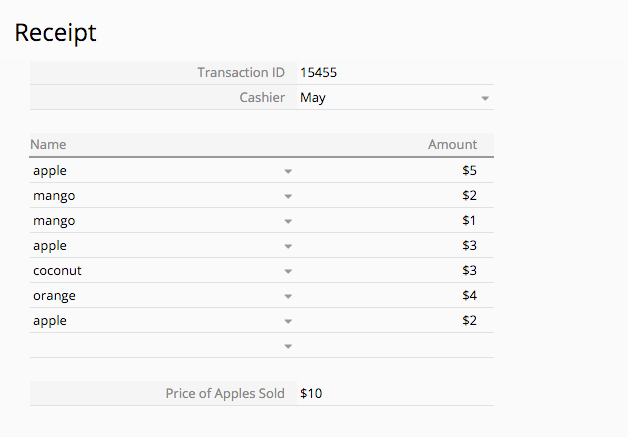
Use COUNTIF to count the number of rows in a Subtable that met a specified criterion; for example, to count the number of times a particular item appears in a receipt.

Formula	Syntax
COUNTIF	COUNTIF(criteria_range,criteria)

Arguments:

criteria_range (required): This range must be a Subtable field to be checked for values that fit specified criteria.

criteria (required): The criteria that defines which cells in criteria_range will be added. This can be a number, expression, reference to another field, or text string that determines which values will be added. Reference the table below:

Application	Examples of Formula Input
Reference Number	"8"
Number Comparison	"> 8"、"< 8"、"!= 8"
Reference Text String	"apple"
String Inequality	"!='apple'"(Use different quotes outside and inside, for example, double quotes outside and single quotes inside)
Reference the Subtable Field	A4 (No need to add double quotes or "="; just write the field name)
Comparison with the Subtable Field	"> A4"、"< A4"、"!=A4"

Note: COUNTIF can only refer to a single Subtable and must be set in independent fields; it supports only one criterion, so use COUNTIFS to apply multiple criteria.

Example:

The Formula COUNTIF(A4,'apple') entered field A9 returns the number of rows that Subtable column A4 contains for the product name apple.

COUNTIFS Function

Formula	Syntax
COUNTIFS	COUNTIFS(criteria_range1,criteria1,[criteria_range2,criteria2]...)

Arguments:

criteria_range1 (required): This range must be a Subtable field to be checked for values that fit specified criteria.

criteria1 (required): The criteria that defines which cells in criteria_range1 will be added. This can be a number, expression, reference to another field, or text string that determines which values will be added. Reference the table below:

Application	Examples of Formula Input
Reference Number	"8"
Number Comparison	"> 8"、"< 8"、"!= 8"
Reference Text String	"apple"
String Inequality	"!='apple'"(Use different quotes outside and inside, for example, double quotes outside and single quotes inside)
Reference the Subtable Field	A4 (No need to add double quotes or "="; just write the field name)
Comparison with the Subtable Field	"> A4"、"< A4"、"!=A4"

criteria_range2, criteria2,... (optional): Rows are counted when additional criteria_ranges match their associated criteria.

Note: COUNTIFS can only refer to a single Subtable and needs to be set in independent fields.

SUMIF Function

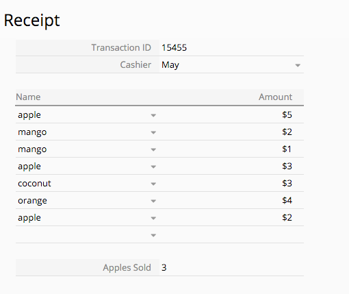
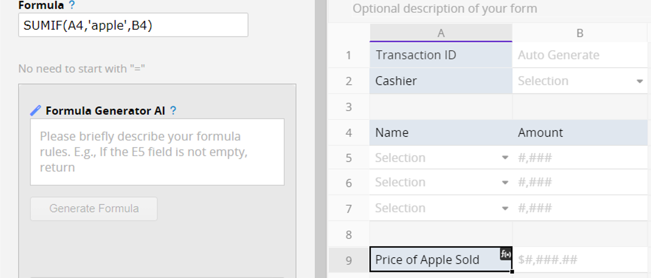
Use SUMIF to sum up the values stored in a specified Subtable row that meet a single criterion; for example, to sum up the monetary value of a specific merchandise item when it appears in a receipt.

Formula	Syntax
SUMIF	SUMIF(range,criteria,[sum_range])

Arguments:

range (required): This range must be a Subtable field to be checked for values that fit specified criteria.

criteria (required)：The criteria that defines which cells in range will be added. This can be a number, expression, reference to another field, or text string that determines which values will be added. Reference the table below:

Application	Examples of Formula Input
Reference Number	"8"
Number Comparison	"> 8"、"< 8"、"!= 8"
Reference Text String	"apple"
String Inequality	"!='apple'"(Use different quotes outside and inside, for example, double quotes outside and single quotes inside)
Reference the Subtable Field	A4 (No need to add double quotes or "="; just write the field name)
Comparison with the Subtable Field	"> A4"、"< A4"、"!=A4"

sum_range (optional)：The actual fields to add, if you want to add values within Subtable fields other than those specified in the range argument. If sum_range is omitted, only the fields that are specified in the range argument will be added (the same fields to which the criteria are applied).

Note: SUMIF can only refer to a single Subtable and must be set in independent fields; it supports only one criterion, so use SUMIFS to apply multiple criteria.

Example:

The Formula SUMIF(A4,'apple',B4) that is entered into field A9 returns the sum of the values in Subtable column B4, when Subtable field header A4 is the product name apple.

SUMIFS Function

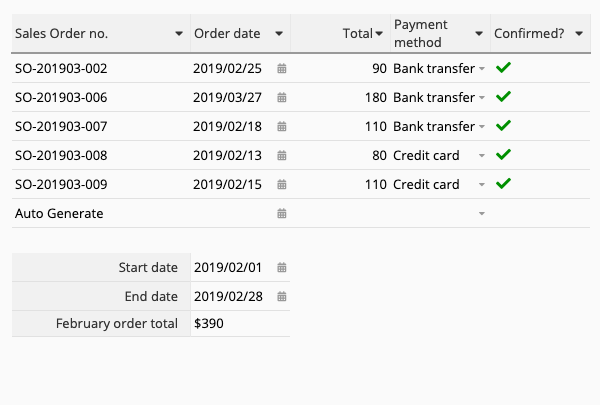
Use SUMIFS to sum up the value stored in a specified Subtable row that meets multiple criteria; for example, to sum up the monetary value of a number of specific merchandise items in specific store locations when it appears in a receipt.

Formula	Syntax
SUMIFS	SUMIFS(sum_range,criteria_range1,criteria1,criteria_range2, criteria2,...)

Arguments:

sum_range (required): This range must be a Subtable field to be checked for values that fit specified criteria.

criteria_range1 (required): criteria_range1 and criteria1 set up a search pair whereby a range is searched for specific criteria. Once items in the range are found, their corresponding values in sum_range are added.

criteria1 (required): The criteria that defines which cells in criteria_range1 will be added. This can be a number, expression, reference to another field, or text string that determines which values will be added. Reference the table below:

Application	Examples of Formula Input
Reference Number	"8"
Number Comparison	"> 8"、"< 8"、"!= 8"
Reference Text String	"apple"
String Inequality	"!='apple'"(Use different quotes outside and inside, for example, double quotes outside and single quotes inside)
Reference the Subtable Field	A4 (No need to add double quotes or "="; just write the field name)
Comparison with the Subtable Field	"> A4"、"< A4"、"!=A4"

criteria_range2,criteria2,... (optional): Additional ranges to be added and their associated criteria.

In the case that you want to apply multiple criteria to a single field, for example, the sum of the A1 field is equal to A or equal to B, you need to use multiple SUMIF() instead of SUMIFS().

Note: SUMIFS can only refer to a single Subtable and needs to be set in independent fields.

Example:

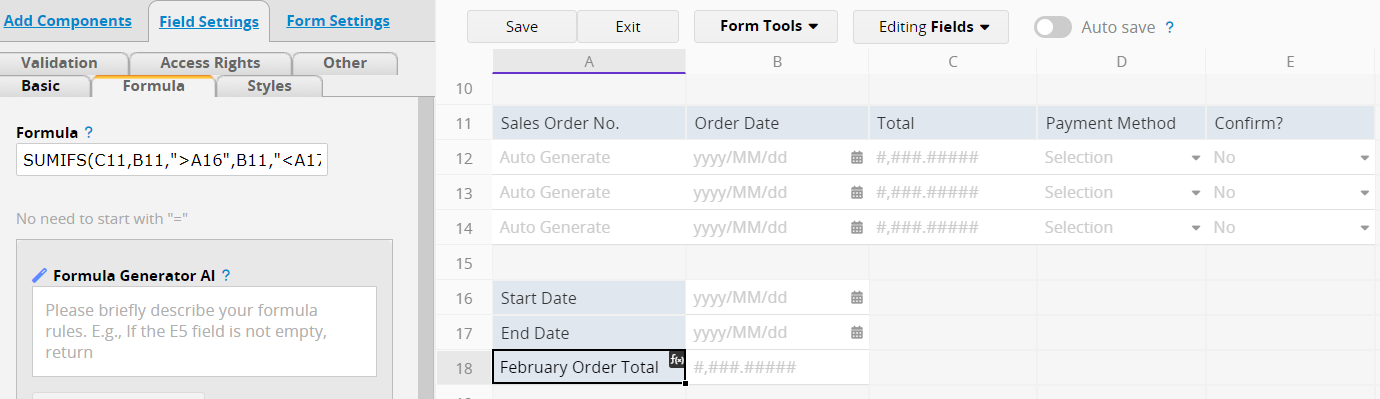
The Formula SUMIFS(C11,B11," > A16",B11," < A17") in the field A18 returns the sum of values Subtable column C11 when the order date (the value B11) is later than that A16 and earlier A17 field.

MAXIFS Function

Returns the maximum value in a range based on one or more criteria, typically used to find the highest price, amount, or most recent date.

Formula	Syntax
MAXIFS	MAXIFS(max_range, criteria_range1, criteria1, [criteria_range2, criteria2], ...)

Arguments:

max_range (required): The Subtable field range to search for the maximum value.

criteria_range1 (required): The first range used to filter matching data.

criteria1 (required): The condition applied to criteria_range1; can be a number, text, or formula.

[criteria_range2, criteria2] (optional): Additional range-condition pairs. Only records meeting all conditions are included in the calculation.

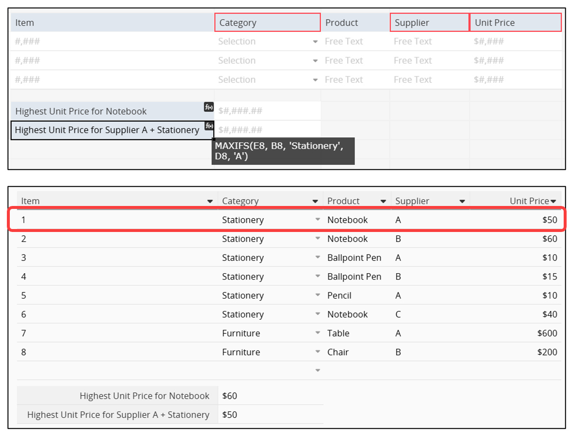
Example 1 (Single Criterion): Find the highest unit price for a specific item.

In the "Quotation Record" sheet, enter MAXIFS("Unit Price", "Item", "Notebook") to find the highest unit price for "Notebook".

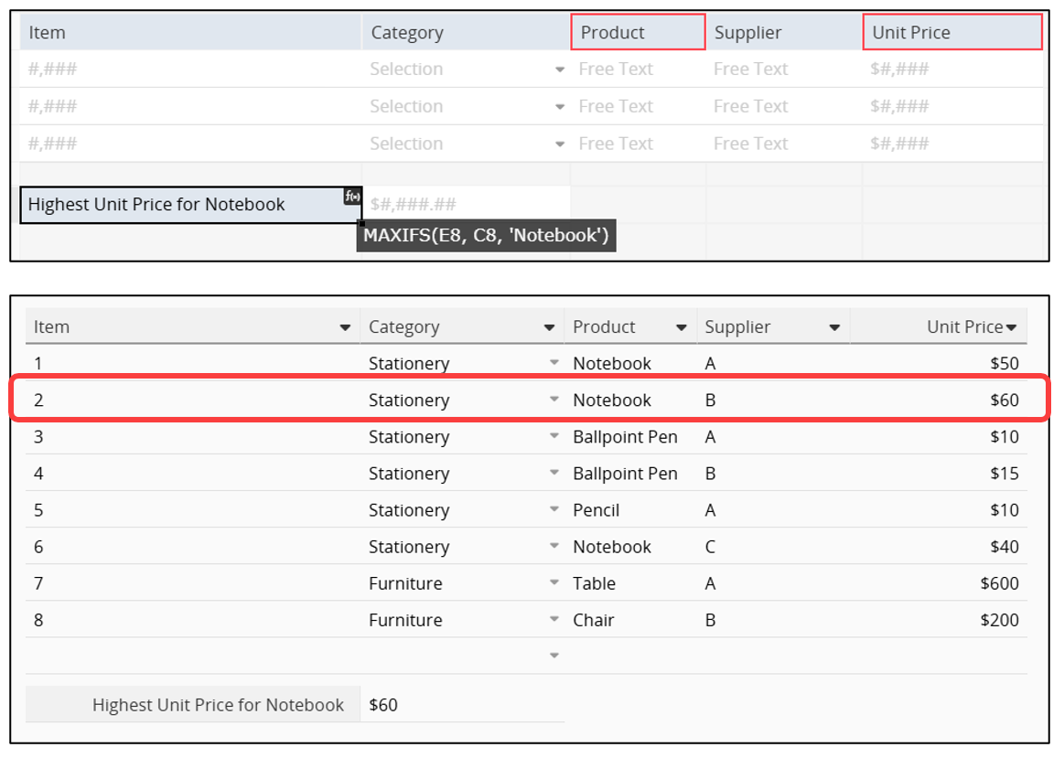
Example 2 (Multiple Criteria): Return the highest unit price by category and supplier. To find the highest unit price where the category is "Stationery" and the supplier is "Supplier A", enter MAXIFS("Unit Price", "Category", "Stationery", "Supplier", "A").

The system returns the highest value among records that meet both criteria.

MINIFS Function

Returns the minimum value in a range based on one or more criteria, typically used to find the lowest price, smallest amount, or earliest date.

Formula	Syntax
MINIFS	MINIFS(min_range, criteria_range1, criteria1, [criteria_range2, criteria2], ...)

Arguments:

min_range (required): The Subtable field range to search for the minimum value.

criteria_range1 (required): The first range used to filter matching data.

criteria1 (required): The condition applied to criteria_range1; can be a number, text, or formula.

[criteria_range2, criteria2] (optional): Additional range-condition pairs. Only records meeting all conditions are included in the calculation.

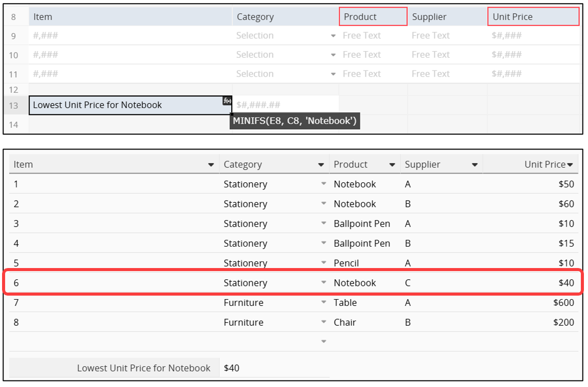
Example 1 (Single Criterion): Find the lowest unit price for a specific item.

In a "Quotation Record" sheet, enter MINIFS("Unit Price", "Item", "Notebook") to find the lowest unit price for "Notebook".

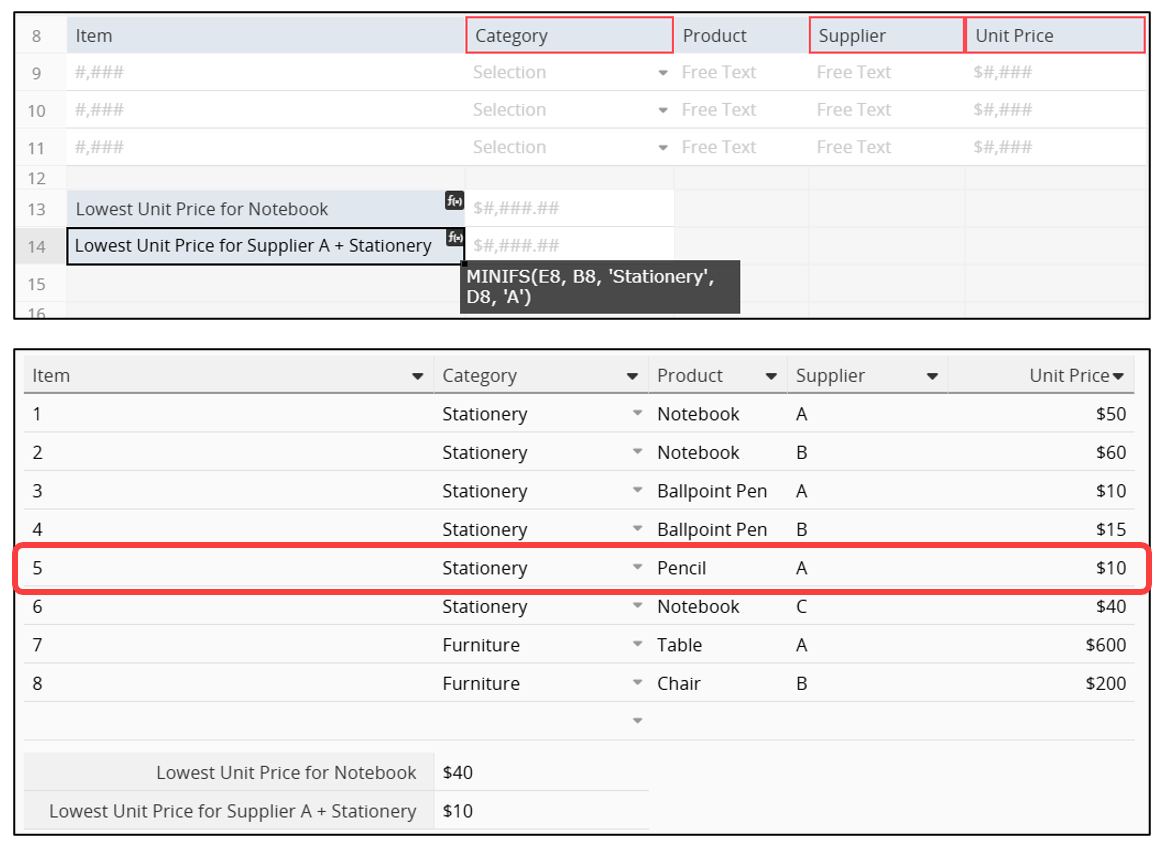
Example 2 (Multiple Criteria): Return the lowest unit price by category and supplier. To find the lowest unit price where the category is "Stationery" and the supplier is "Supplier A", enter: MINIFS("Unit Price", "Category", "Stationery", "Supplier", "A").

The system will return the lowest value among records that meet both conditions.

Nesting Conditional Formulas

Conditional formulas can be nested when multiple conditions must be met.

Example 1:

IF(A1==1,'Bad',IF(A1==2,'Good',IF(A1==3,'Excellent','No Valid Score')))

The above formula means that:

if A1 is 1, the result is "Bad".

if A1 is 2, the result is "Good".

if A1 is 3, the result is "Excellent".

if A1 is anything else, the result would be "No Valid Score".

Example 2:

IF(
AND(A1.RAW=='YES',A2.RAW=='Jimmy'),
C3*C7,
IF(
AND(A1.RAW=='YES',A2.RAW=='John'),
C3*C8,
IF(
AND(A1.RAW=='YES',A2.RAW=='Jane'),
C3*C9,
C3*C10
)
)
)

The above formula means that:

if A1 has the value "YES", and A2 has the value "Jimmy", the result is C3*C7.

if A1 has the value "YES", and A2 has the value "John", the result is C3*C8.

if A1 has the value "YES", and A2 has the value "Jane", the result is C3*C9.

if these conditions do not apply, then the result is C3*C10.

IFS Function

In addition to the nested conditional formulas, you can also use IFS() to check whether one or more conditions are met, and return a value that corresponds to the first TRUE condition.

Formula	Syntax
IFS()	IFS(value=condition1,value_if_true1,value=condition2,value_if_true2, ...,true,default value)

Arguments:

value=condition1 (required): The first condition evaluates to TRUE or FALSE.

value_if_true1 (required): Result to be returned if value=condition1 evaluates to TRUE.

value=condition2 (required): The second condition evaluates to TRUE or FALSE.

value_if_true2 (required): Result to be returned if value=condition2 evaluates to TRUE.

*You need to set at least two sets of conditions. You can apply more if needed.

true (optional): Please input "true" if you want to set the default value when none of the other conditions are met.

default value (optional): The result is returned if none of the other conditions are met.

Example:

 
IFS(A1=1,"Bad",A1=2,"Good",A1=3,"Excellent",true,"No Valid Score") 

The above formula means that:

if A1 is 1, the result is "Bad".

if A1 is 2, the result is "Good".

if A1 is 3, the result is "Excellent".

if A1 is anything else, the result would be "No Valid Score".

Other Formula Details and Applications

LOOKUP Function

Returns the corresponding result based on a specified range or condition.

Formula	Syntax
LOOKUP	LOOKUP(value,lookup_list,[result_list])

value (required): The field value to search for. The system looks for an exact or closest match in the lookup_list.

[lookup_list] (required): An array such as [0, 100, 500] where LOOKUP searches for the specified value.

result_list (optional): Defines the results to return when a match is found. It must match the number of items in lookup_list, for example ["Small", "Medium", "Large"]. If omitted, the function returns the value from lookup_list or, if no exact match is found, the result for the largest value less than or equal to the specified value. Returns blank if smaller than all items.

Examples 1: LOOKUP(A1,[0,45,65],['Small','Medium','Large'])

The value would be 'Small' if the value of A1 is between 0 and 44, 'Medium' for 45~64, and 'Large' for greater than or equal to 65.

Examples 2 (Referencing multiple fields): LOOKUP(A1,[0,45,65],[A3+A4,B5,B6])

The value would be A3+A4 if the value of A1 is between 0 and 44, B5 for 45~45, and B6 for greater than or equal to 65.

AND Function

Returns TRUE if all test conditions evaluate to TRUE; returns FALSE if one or more conditions evaluate to FALSE.

Formula	Syntax
AND	AND(logical1, [logical2], ...)

Arguments:

logical1 (required): The first condition to be tested, which returns either TRUE or FALSE.

logical2 (optional): Additional conditions that also affect whether the result is TRUE or FALSE.

OR Function

Returns TRUE if any test condition is TRUE; returns FALSE if all conditions are FALSE.

Formula	Syntax
OR	OR(logical1, [logical2], ...)

Arguments:

logical1 (required): The first condition evaluated as either TRUE or FALSE.

logical2 (optional): Additional conditions; if any evaluate to TRUE, the overall result returns TRUE.

NOT Function

Returns TRUE if the test condition is FALSE, and FALSE if the condition is TRUE.

Formula	Syntax
NOT	NOT(logical)

Example:

NOT(A2>10)

If the value in reference field A2 is less than or equal to 10, the system returns "true"; otherwise, it returns "false".

UPDATEIF Function

Use UPDATEIF to retain the old value in the field if the condition is false. The value in a field where the UPDATEIF function is used should change only if the condition being tested by the UPDATEIF Function is true.

Formula	Syntax
UPDATEIF	UPDATEIF(condition,value_if_true)

Arguments:

condition (required): Determines whether the field is updated. If the condition is met, the field is updated; otherwise, it stays the same.

value_if_true (required): The value to apply when the condition is met, which can be a number, text, or another field reference.

Examples:

Basic Example: UPDATEIF(A2==10,10)

If the value in the reference field A2 is equal to 10, the value in this field would be 10. For any other value of A2, the value of this field would remain unchanged from the previously saved version of the record.

Practical Example: UPDATEIF(A2=='Same as home address',A1)

If the value in field A2 is 'Same as home address', the value in the field "Shipping address" would be A1 (home address); otherwise, the value would remain empty.